Two weeks ago, I challenged readers to reproduce a circle chart from Innovation Network’s State of Evaluation 2012 report — using only Microsoft Excel or R. You can read the full blog post here.
And the winners are… Tony Fujs, Andrea Hutson, Prince Rajan, and Bernadette Wright! Tony re-created the chart in R, and Andrea, Prince, and Bernadette re-created the chart in Excel.
Here’s my how-to guide. At the bottom of this blog post, you can download an Excel file that contains each of the submissions. We each used a slightly different approach, so I encourage you to study the file and see how we manipulated Excel in different ways.
Step 1: Study the Chart that You’re Trying to Reproduce in Excel
Here’s that chart from page 7 of the State of Evaluation 2012 report. We want to see whether we can re-create the chart in the lower right corner. The visualization uses circles, which means we’re going to create a bubble chart in Excel.
Step 2: Learn the Basics of Making a Bubble Chart in Excel
To fool Excel into making circles, we need to create a bubble chart in Excel. Click here for a Microsoft Office tutorial. According to the tutorial, “A bubble chart is a variation of a scatter chart in which the data points are replaced with bubbles. A bubble chart can be used instead of a scatter chart if your data has three data series.”
We’re not creating a true scatter plot or bubble chart because we’re not showing correlations between any variables. Instead, we’re just using the foundation of the bubble chart design – the circles. But, we still need to envision our chart on an x-y axis in order to make the circles.
Step 3: Sketch Your Chart on an X-Y Plane
It helps to sketch this part by hand. I printed page 7 of the report and drew my x and y axes right on top of the chart. For example, 79% of large nonprofit organizations reported that they compile statistics. This bubble would get an x-value of 3 and a y-value of 5.
I didn’t use sequential numbering on my axes. In other words, you’ll notice that my y-axis has values of 1, 3, and 5 instead of 1, 2, and 3. I learned that the formatting seemed to look better when I had a little more space between my bubbles.
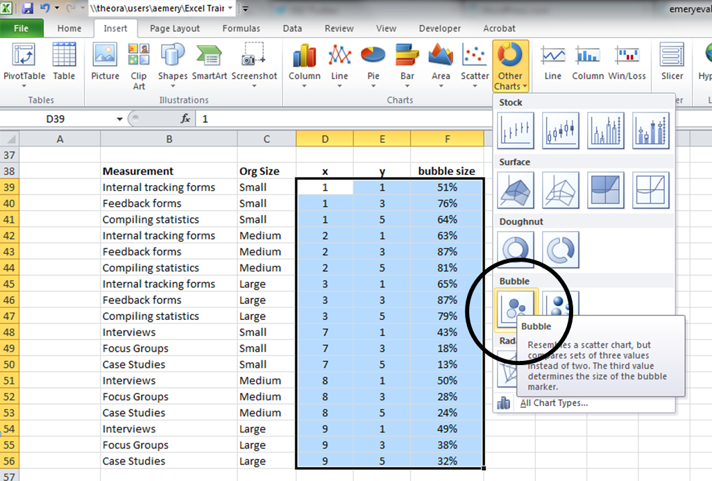
Step 4: Fill In Your Data Table in Excel
Open a new Excel file and start typing in your values. For example, we know that 79% of large nonprofit organizations reported that they compile statistics. This bubble has an x-value of 3, a y-value of 5, and a bubble size of 79%.
Go slowly. Check your work. If you make a typo in this step, your chart will get all wonky.
Step 5: Insert a Bubble Chart in Excel
Highlight the three columns on the right – the x column, the y column, and the frequency column. Don’t highlight the headers themselves (x, y, and bubble size). Click on the “Insert” tab at the top of the screen. Click on “Other Charts” and select a “Bubble Chart.”
You’ll get something that looks like this:
Step 6: Add and Format the Data Labels
First, add the basic data labels. Right-click on one of the bubbles. A drop-down menu will appear. Select “Add Data Labels.” You’ll get something that looks like this:
Second, adjust the data labels. Right-click on one of the data labels (not on the bubble). A drop-down menu will appear. Select “Format Data Labels.” A pop-up screen will appear. You need to adjust two things. Under “Label Contains,” select “Bubble Size.” (The default setting on my computer is “Y Value.”) Next, under “Label Position,” select “Center.” (The default setting on my computer is “Right.)
Step 7: Format Everything Else
Your basic bubble chart is finished! Now, you just need to fiddle with the formatting. This is easier said than done, and probably takes the longest out of all the steps.
Here’s how I formatted my chart:
- I formatted the axes so that my x-values ranged from 0 to 10 and my y-values ranged from 0 to 6.
- I inserted separate text boxes for each of the following: the small, medium, and large organizations; the quantitative and qualitative practices; and the type evaluation practice (e.g., compiling statistics, feedback forms, etc.) I also made the text gray instead of black.
- I increased the font size and used bold font.
- I changed the color of the bubbles to blue, light green, and red.
- I made the gridlines gray instead of black, and I inserted a white text box on top of the top and bottom gridlines to hide them from sight.
Your final chart will look something like this: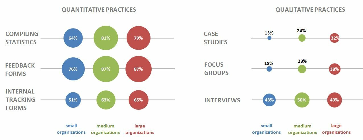
Bonus! Download the Excel File
Click below to download the Excel file that I used to create this bubble chart. Please explore the chart by right-clicking to see how the various components were made. You’ll notice a lot of text boxes on top of each other!
Download the Excel FileThanks again to the dataviz challenge winners, Tony Fujs, Andrea Hutson, Prince Rajan, and Bernadette Wright! Tony, Andrea, Prince, and Bernadette have graciously shared their Excel files. I created a separate tab to showcase each of their charts. We each formatted the data table and the chart a little differently, so I encourage you to explore their approaches and contact them with additional questions (and kudos!).
7 Comments
Great idea for a competition. I couldn’t help myself but try to figure it out too. I was interested to see how you managed to remove the axis and replace them with text – it would be great if Excel allowed you to have arbitrary axis labels.
Greetings Matt,
Thanks for your interest in the competition! I hope you learned new skills and had fun with it.
You can definitely remove the default axis and axis labels in Excel and replace them with text boxes instead. Text boxes are becoming more and more popular. Having control over your axes allows you to make the graphic easier to read and understand. I’ll either make a video tutorial or add details to this blog post to give you more behind-the-scenes details so you can follow along and try it for yourself.
Thanks again for participating and trying it out yourself!
Ann
Hello, Ann,
I follow your blog as it is reposted in Eval Central. I also blog (Evaluation is an everyday activity; http://blogs.oregonstate.edu/programevaluation/)and am interested in building evaluation capacity for Extension professionals. Your challenge and answer are just the kind of information I would love to share with my audience. I’d credit you. Would you mind.
Molly Engle.
Molly,
Thanks for following. I follow your blog as well. Nice to officially “meet” you virtually!
Feel free to share any and all resources with your Extension professionals. I also make video tutorials that you can share with others (http://emeryevaluation.com/excel/). The videos focus on beginner-level foundational skills. I’ll probably share a dataviz challenge every month or every other month for folks who are ready for intermediate and advanced skills.
Thanks again for following,
Ann
[…] to everyone who participated in the first and second dataviz challenges! I hope these challenges give you a chance to practice and build upon […]
[…] Rad Resource: Want to learn how to make bubble charts? Check out Ann Emery’s blog to get help on constructing circle charts. […]
[…] circle chart/area chart to show the countries represented. (Charts that display differences through a […]