
Vlookup is my all-time favorite function in Excel!
(Well, the entire lookup family—vlookup, hlookup, index-match, and xlookup.)
In this blog post, you’ll learn:
- What vlookup is used for;
- Why vlookup can be tricky; and
- How to fill in the four pieces of the formula.
What Vlookup Is Used for in Excel
Vlookup helps us merge data from various tables, sheets, and files into a single table that we can use for our analyses.
Why Vlookup is Tricky for Novices
Sometimes Excel novices are hesitant to try vlookup because it requires that you fill in four different pieces of information.
Learning the Excel lingo here is truly like learning a new language. Stick with it and keep practicing, and you’ll be a fluent vlookup user in no time!
Here’s the information that we’ll need to complete: =vlookup(lookup_value,table_array,col_index_num,[range_lookup])
Let’s walk through each of the four segments of the vlookup function.
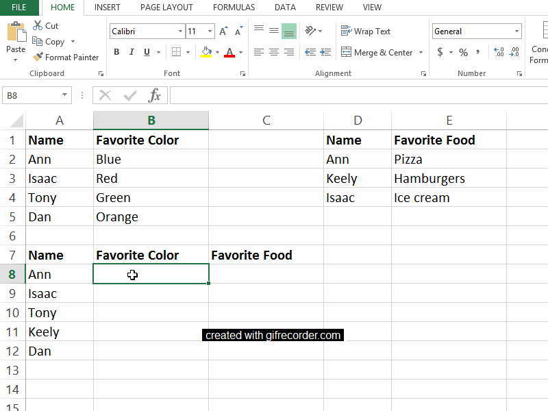
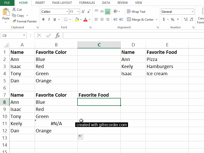
Our Fictional Scenario
I’ve got five people: Ann, Isaac, Tony, Keely, and Dan. I’ve also got two different tables of data: Favorite Color and Favorite Food.
Let’s pretend I want to create a single dataset that contains both the colors and the foods together.
In a perfect world, I’d be able to copy and paste the colors and foods together.
But in the real world, we’ve typically got different numbers of people in each of the original tables. For example, we’ve got information about Ann, Isaac, Tony, and Dan in our Favorite Color table, but we’ve only got information about Ann, Keely, and Isaac in our Favorite Food table, so a simple copy and paste isn’t possible.
Sure, with just five people, we could fill in this information by hand. But what if our dataset contains information about 50 people? Or 50,000 people? Copying and pasting could take all day, and we’d probably make a million mistakes along the way. Vlookup to the rescue!
How to Use =Vlookup() in Microsoft Excel
Here’s how to fill in each of the four pieces of the vlookup formula.
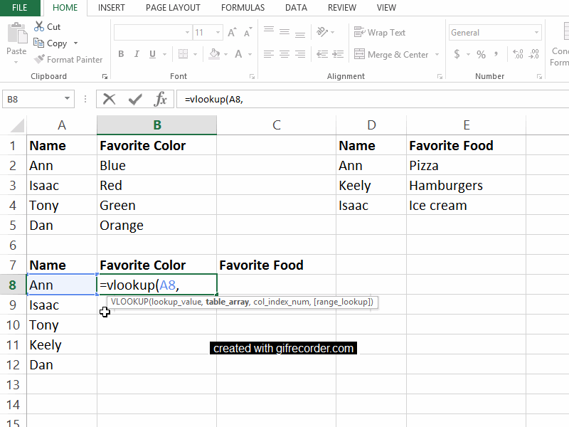
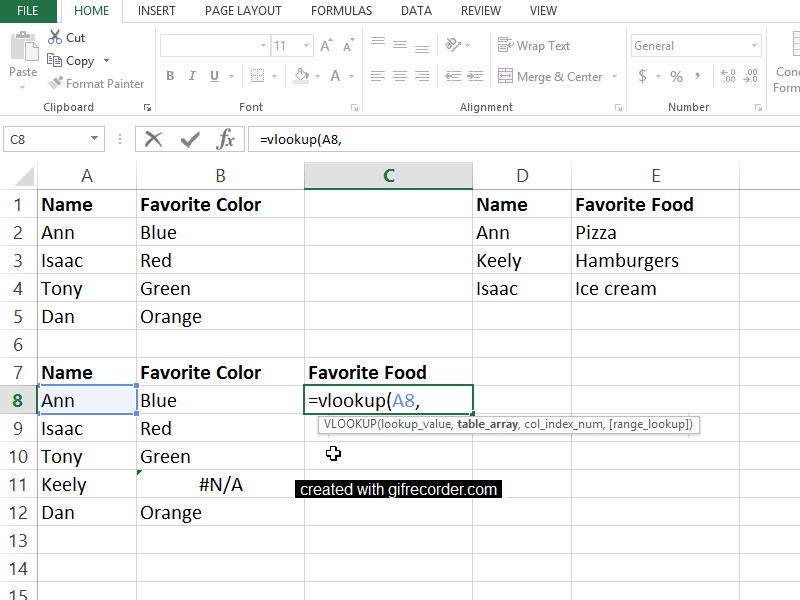
Step 1: Fill in the lookup_value
First, let’s fill in the lookup_value, which is the first piece of the vlookup function.
The lookup_value is the cell that contains the person’s name or ID number that we’re interested in. These names or ID numbers are the links that connect all the tables together.
The names or ID numbers must be located in the first column of each table–in the first column of your new combined dataset and in the first column of every single table from which you’re pulling data.
In this example, watch as I type =vlookup( into cell B8. Next, click on the cell that contains the name or ID number that you want to look up in one of your other tables. Then, insert a comma, which moves us on to the second section of the function.
So far, my function reads: =vlookup(A8,
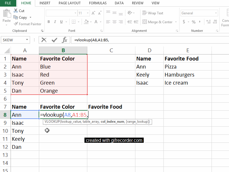
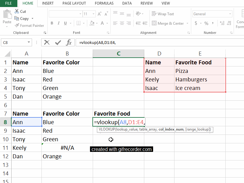
Step 2: Fill in the table_array
Second, we have to indicate the table_array.
The table array is the table or dataset from which we’re pulling data.
In this example, we want to get information from the Favorite Color table into our master table down below. The table_array for the Favorite Color table is A1:B5. In other words, that table begins in cell A1 and ends in cell B5.
My function reads: =vlookup(A8,A1:B5,
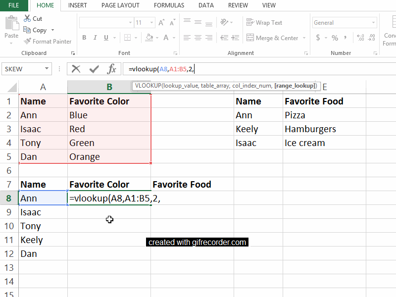
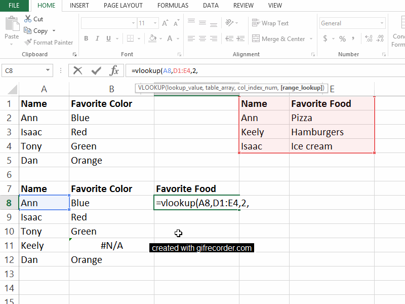
Step 3: Fill in the col_index_num
Third, we have to indicate the col_index_num.
This column index number is the number of the column we care about. Just type in the number of the column you’re interested in.
For example, we want to know favorite colors, which are located in the second column of our Favorite Color table, so we type a 2 into the vlookup function. As usual, conclude with a comma to move on to the fourth and final segment of our function.
My function reads: =vlookup(A8,A1:B5,2,
Step 4: Fill in the range_lookup
Fourth, we need to indicate the range_lookup..
We have to type the word true or false into the fourth and final section of our vlookup function.
A true will give us an approximate match and a false will give us the exact information we’re looking for. We obviously want precise information, so type false into the function and end with a closing parenthesis.
My completed function reads: =vlookup(A8,A1:B5,2,false)
We can see that Ann’s favorite color is blue.
A Second Vlookup Example
Let’s go through a second vlookup example to make sure the four pieces of the function make sense.
We’ll continue creating a master table that combines content from both the Favorite Color and Favorite Food tables into a single table.
First, in cell C8, type =vlookup(A8, to set the lookup_value as Ann.
Second, indicate the boundaries of the Favorite Food table that we want to pay attention to. My function now reads =vlookup(A8,D1:E4
Third, tell Excel which column of the Favorite Food table to focus on. The foods are listed in the second column of that mini-table, so enter a 2 into the vlookup function. My function says =vlookup(A8,D1:E4,2
Finally, type false into the function and close your parentheses. The completed function says =vlookup(A8,D1:E4,2,false) and tells us that Ann’s favorite food is pizza.
Vlookup takes time to sink in, so go easy on yourself if you don’t “get it” right away. I promise that the time-savings from vlookup are worth the learning curve.
4 Comments
Have you explored XLOOKUP yet? It’s like the glow-up version of VLOOKUP. Simple – powerful – and solves many of the potential pitfalls of using vlookup in changing spreadsheets.
Yes, love it! I haven’t officially blogged on it yet because it’s new-ish (early 2020 release, I think). I work with a lot of government employees, nonprofit staff, and university staff who might not have the latest version of Excel, so I like to wait a bit to talk about new features so that they don’t feel left out.
The methods is good
Do you click and drag to expand the formula to all participants ?