Want to make an interactive dashboard in Microsoft Excel?
Interactive (a.k.a. dynamic) dashboards are a great option for technical audiences that have the time and interest to explore the data for themselves.
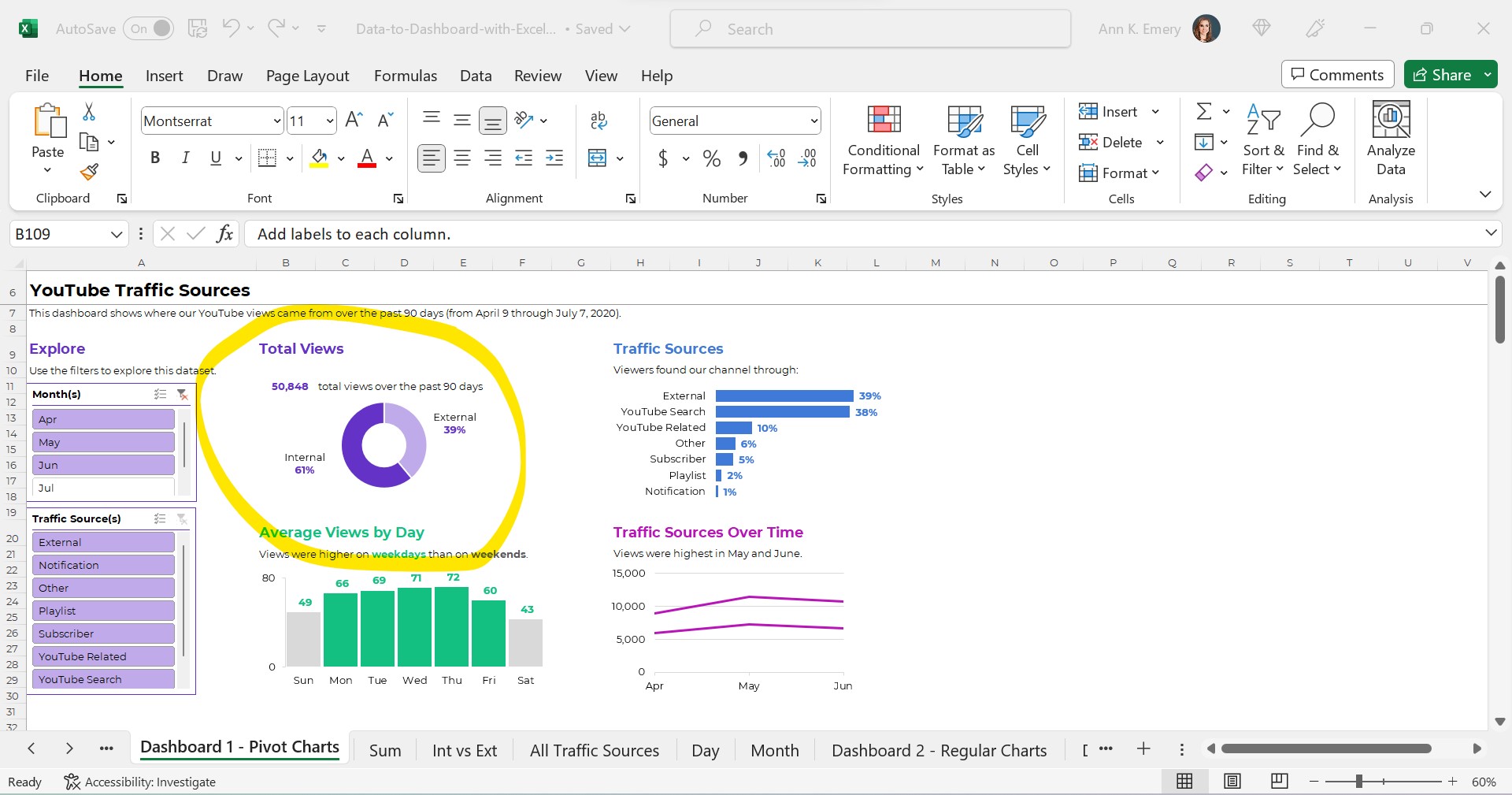
They’ll look something like this:

Interactive dashboards are easy to create — sort of. It depends on your existing skill level.
You’ll need four pieces:
- A Clean, Contiguous Dataset (maybe stored as an Excel Table)
- Pivot Tables
- Pivot Charts
- Slicers
Are you already using these four features regularly? Great! Linking them together in a dashboard will be easy for you.
Are you new to Excel Tables, pivot tables, pivot charts, or slicers? Be patient with yourself. You’ll need to be fluent in the building blocks before you can put them together seamlessly.
Let’s walk through each of the four pieces in more detail.
Step 1: Build the Clean, Contiguous Dataset
From previous blog posts, you know that table is a tricky term.
There are several different types of tables, like datasets vs. tabulations. In short, a dataset is the underlying numbers, and the tabulation is the summary table.
The Raw Dataset
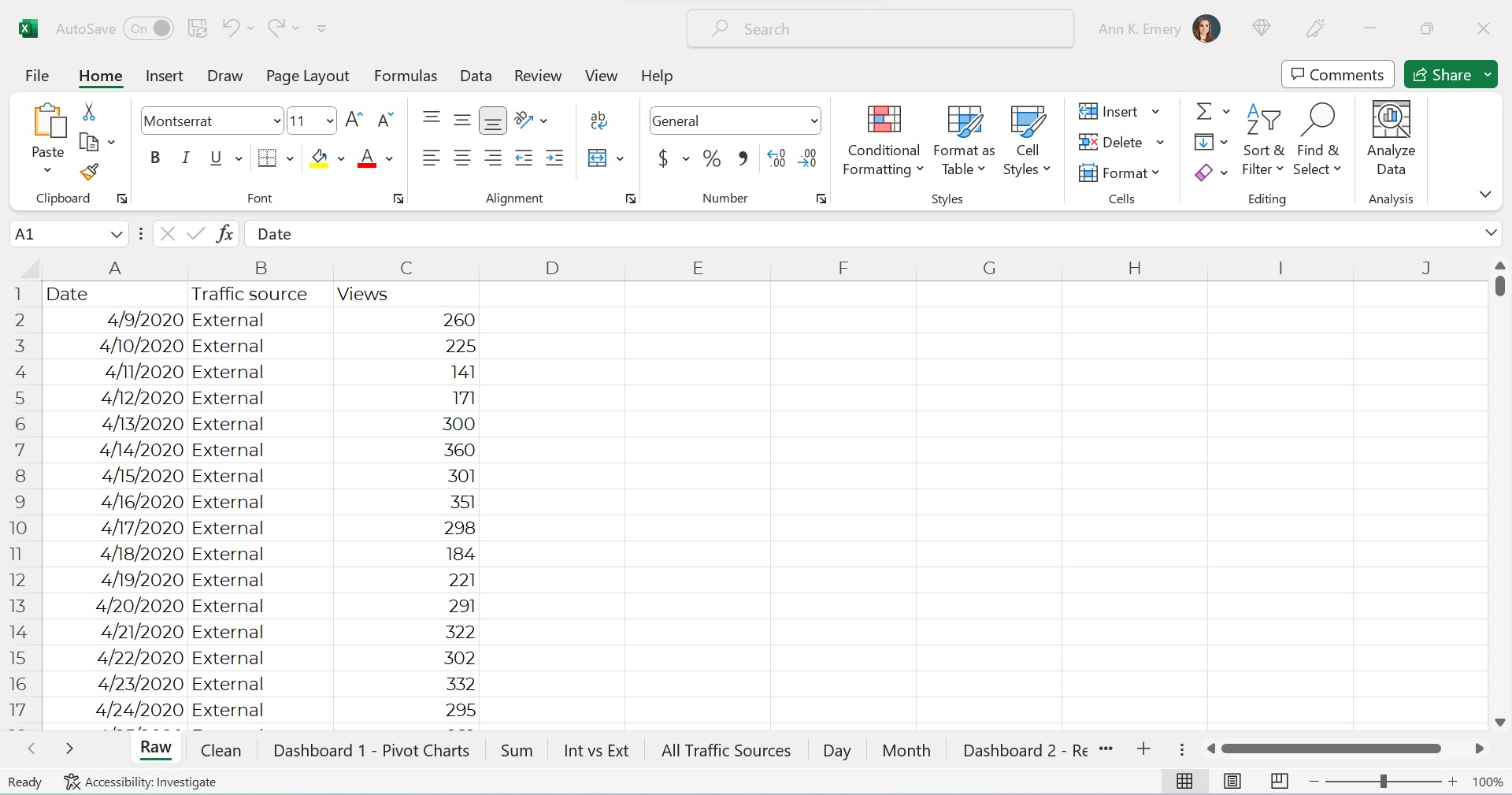
To build our interactive dashboard, we’ll start with our raw dataset.
This is semi-fictional data. We’re pretending that we’ve downloaded YouTube stats directly from YouTube.
The raw dataset would look something like this, with one entry per date and traffic source.
It’s raw because this is exactly what it looks like when downloaded from YouTube. We haven’t made any changes (yet!).
The Clean Dataset
Next, we’d clean the dataset.
We might check for and deal with duplicates.
We might check for and deal with missing data.
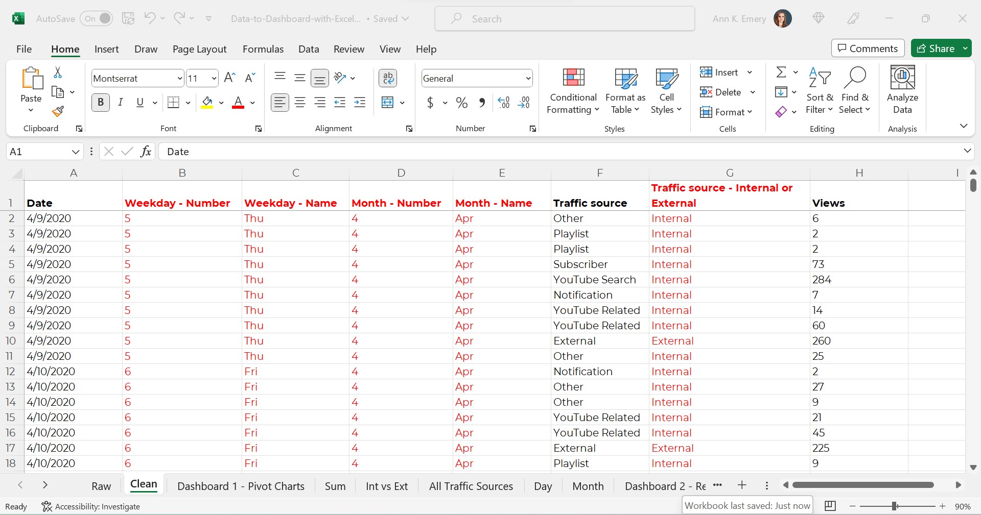
We might add lots of new columns of recoded data. For example, if I want to make a donut chart comparing the internal and external traffic sources, then I’ll need a column (a variable) that categorizes each traffic source as being internal or external.
If I want to make a graph that compares YouTube visits by day of the week (Monday vs. Tuesday views), then I’ll need a column that turns MM/DD/YYYY into weekday. And so on.
(You can learn more about cleaning, recoding, and transforming datasets inside Simple Spreadsheets, my prerequisite course. Again, you’ll need to be 100% fluent in these skills. Otherwise, dashboards will feel daunting.)
Years ago, a coworker taught me to turn all my new variables red so my Future Self could find them. As you can see, I still follow that advice today.
The clean dataset would look something like this:
Required: A Contiguous Dataset
As usual, my clean dataset is contiguous.
In other words, all the cells are touching or sharing a border.
I don’t have dozens of mini datasets (like one per month, or one per traffic source).
You can learn more about contiguous datasets and why they’re necessary for dataviz in this blog post.
Optional: An Excel Table
Next, we might transform our clean dataset into an Excel Table. This step is optional.
As explained in this blog post, Excel Tables are helpful when we need to append tables (that is, when we’ll be adding more rows over time).
Alright, that’s it for the first piece! We’ve got a single, clean, contiguous dataset as our base. We might store it as a regular ol’ table/dataset. Or, we might turn it into an Excel Table for easy appending.
Step 2: Tabulate the Dataset with Pivot Tables
We can tabulate our dataset with either (1) formulas or (2) pivot tables. You can learn more about the pros and cons of each approach in this blog post.
In short, if we’re aiming to build an interactive dashboards… which has to involve slicers… which have to involve pivot charts… then we simply have to use pivot tables.
Again, interactive dashboards are easy — sort of. You have to understand all the nuances of when to use regular ol’ tables vs. Excel Tables, and when to formulas vs. pivot tables, in order to work both backwards and forwards and put everything together quickly and correctly.
Our pivot tables will look something like this:
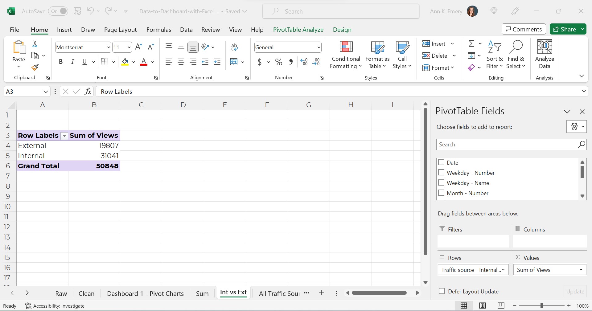
Interactive dashboards involve pivot tables — plural.
We’ll need one pivot table for each of our charts.
In the finished example, there were four charts + a sum of the total views. That means there are five separate pivot tables behind the scenes.
If you’re familiar with pivot tables, great! Building a few pivot tables for your dashboard will be easy.
If you’re brand new to pivot tables, no worries! I’ve got plenty of beginner-level blog posts to get you started.
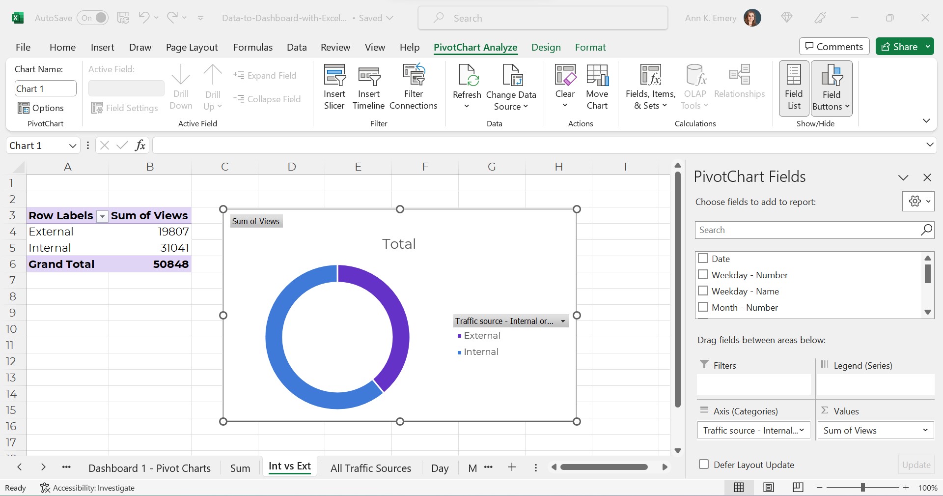
Step 3: Build (and Format) the Pivot Charts
Next, we’ll simply add a pivot chart to each of our pivot tables.
In case you’re brand new to pivot charts, here’s how you add them:
- Click on the pivot table to activate it.
- Go to the Insert tab.
- Choose which chart type you’d like (bar, line, donut, etc.).
- That’s it!
Please, don’t forget the formatting!!!
Our unformatted chart — which doesn’t pass 508/ADA compliance guidelines — would look like this:
The formatted chart would look like this.
Do you notice the binary color-coding, white outlines around touching shapes, and the direct labels?
Once we’ve built and formatted each of the charts, we’ll simply cut and paste them together into a new sheet. That’s where our soon-to-be-completed dashboard will live.
Step 4. Add a Slicer(s)
Finally, we’ll add a slicer(s) to the first pivot chart.
A slicer is just a fancy name for a filter. They’ve existed in Excel since 2010 (!!!). But, don’t worry if you haven’t seem them or used them before. It takes years for new features to be widely adopted. (Hence the point of blog posts like these — to introduce you to features you might not have discovered before.)
Connect the Slicer to the First Chart
In case you’re brand new to slicers, here’s how you add them:
- Click on one of the pivot charts to activate it.
- Go to the Insert tab.
- Click on the Slicer option.
- You’ll see a list of all the variables. In this example, our variables from the clean dataset are Date, Weekday – Number, Weekday – Name, Month – Number, Month – Name, Traffic Source, Traffic Source – Internal or External and Views. If I want viewers to be able to slice and dice by month, then I’d select Month – Name to feed into the slicer.
- That’s it!
Connect the Slicer to the Rest of the Charts
The slicer won’t automatically be connected to all of our charts.
We’ll need one more step:
- Click on the slicer to activate it.
- Go to the Slicer tab.
- Click on the Report Connections button.
- We’ll see a list of all our pivot tables. Check all the boxes.
- That’s it! Now, when we filter data with the slicer, all the charts will correctly filter and change, too.
Final Formatting
As usual, we’ll make sure to follow dataviz best practices.
We’ll need to:
- Add words. We’ll need a title, date, subtitles, and explanatory text. Yes, there’s concatenation behind the scenes that automatically writes the sentences for me.
- Use brand colors and brand fonts.
- Color-code by category. (One brand color per category/section/chart.)
- Leave plenty of white space between the charts. My rule of thumb: A thumb’s width (a half-inch or inch of white space between each chart).
Now it’s time to sit back, relax, and let our colleagues have fun exploring the dashboard for themselves.
Learn More
If this tutorial is easy for you, then congrats!!! You’re all set. Go forth and build magnificent, accessible, interactive dashboards for your technical-minded colleagues.
If this tutorial was jargony for you, don’t worry!!! You can walk through each of the steps in more detail, and download the spreadsheets to follow, and come to live Office Hours inside the Dashboard Design course.
2 Comments
You mention that you use concatenate at the end to add words. Is there a way to make the words change as they use the slicers?
I want file exel